The project began as a scraper. It became more useful when I treated the resulting archive as a measurement system: a way to ask what separates two newsrooms, how much of that difference is topic rather than style, and whether a model can reproduce the distinction.

The analysis uses 2,304 articles published in January 2026: 1,963 from N1 Srbija and 341 from Biznis.rs. I developed it across three machine-learning assignments. They overlap heavily, so this page presents them as one cumulative study rather than three separate papers.

The collected corpus was not balancedArticles published in January 2026

N1 Srbija85.2% of the corpus

1963 articles

Biznis.rs14.8% of the corpus

341 articles

How the three iterations fit together

Iteration	New question	Main addition
1	Can article text identify the outlet?	TF-IDF, logistic regression, Naive Bayes, LinearSVC
2	How much can the representation be compressed?	LSA and a neural autoencoder
3	What signal is the classifier actually using?	BERTić, metadata ablation, NMF topics, retrieval, and mT5 generation

The corpus, preprocessing, TF-IDF baseline, and most of the evaluation machinery recur in all three. The real progression is from prediction, to compression, to interpretation.

The question kept changing

I did not begin with a theory about editorial style. I began with a practical annoyance: collecting articles from different sites produces records that look similar but are never quite interchangeable. Each source has its own page structure, naming conventions, missing fields, and repeated boilerplate. Building the scraper forced me to decide what an article actually is before I could analyze one.

Once the data was clean enough to compare, the first classification score was almost suspiciously high. That changed the project. “Can a model distinguish the outlets?” was no longer a very interesting question; clearly it could. The better question was why it could. Was it learning writing style, subject matter, author signatures, page furniture, or some mixture of all four?

Each iteration therefore tried to remove one easy explanation. The first established a careful baseline under class imbalance. The second asked whether the signal was spread across thousands of terms or concentrated in a much smaller space. The third opened the model up: remove metadata, inspect coefficients and topics, compare contextual embeddings, and finally ask whether the learned distinction could be controlled during generation.

From web pages to a corpus

Two Scrapy spiders walk each outlet's archive, follow article pages, and emit the same record shape for title, URL, timestamp, category, author, body, images, and embedded media. Source-specific parsing stays inside the collector. Downstream analysis sees one stable table.

That separation is the part of the engineering I care about most. A crawler should be allowed to break when a publisher changes its markup without forcing every later notebook to change with it. The normalized article record became the boundary between acquisition and analysis. It also made failures visible: an empty author is a missing value; an empty body is a broken extraction.

The imbalance is substantial: N1 supplied almost six times as many articles. Biznis articles were also longer at the median: 2,607 characters versus 1,574 for N1. That matters because an apparently strong classifier can simply learn the majority class or other collection artifacts.

For classical models, I joined paragraphs, lowercased and normalized Serbian text, transliterated Cyrillic to Latin, removed Serbian stopwords, and built unigram and bigram TF-IDF features. A typical article activates only a tiny fraction of the roughly 39,000 resulting features.

Transliteration was a modeling choice, not just cleaning. It stops the same Serbian word written in two scripts from becoming two unrelated features, but it also removes script choice as a possible editorial signal. I accepted that trade-off because I wanted the first model to compare vocabulary rather than typography. Bigrams remained useful because phrases such as institutional names and market expressions carry more information than their individual words.

The weight of term $t$ in document $d$ is:

$$\operatorname{tfidf}(t,d) = \bigl(1+\log f_{t,d}\bigr) \log\left(\frac{N}{1+\operatorname{df}(t)}\right)$$

This deliberately simple representation preserves the lexical choices that turned out to matter most.

An honest evaluation contract

The first iteration used stratified five-fold cross-validation, then reduced the N1 class inside each training fold only. The validation fold kept the original 6:1 prevalence. Ten resamples per fold produced 50 fits per configuration.

The order is important. Balancing the whole dataset before splitting would make evaluation easier and would no longer answer how the model behaves on the distribution it will actually see. Resampling only the training fold gives the learner equal exposure to both outlets while leaving the test unchanged. Repeating the random undersampling also reveals whether a result depends on one fortunate selection of N1 articles.

for train_idx, val_idx in folds.split(X, y):
    minority = train_idx[y[train_idx] == "biznis"]
    majority = train_idx[y[train_idx] == "n1"]

    sampled = rng.choice(
        majority,
        size=len(minority),
        replace=False,
    )
    balanced_train = np.r_[minority, sampled]

    model.fit(X[balanced_train], y[balanced_train])
    predictions = model.predict(X[val_idx])

Because accuracy can hide minority-class failure, I used macro F1 as the primary score:

$$F_1^{\mathrm{macro}} = \frac{F_{1,\mathrm{N1}}+F_{1,\mathrm{Biznis}}}{2}, \qquad F_1=2\frac{\mathrm{precision}\cdot\mathrm{recall}} {\mathrm{precision}+\mathrm{recall}}.$$

There is one important wrinkle. The later two assignments first created a balanced 682-article working set and then split it into folds. That is a different, easier evaluation distribution. The original run produced macro F1 0.9685; the later shared comparison pipeline produced 0.9880. I do not treat that increase as a model improvement. I use 0.9880 only when comparing representations evaluated under the same later protocol.

This is also why I report the protocols rather than one “best” number. A score is partly a property of the model, but it is also a property of the split, prevalence, preprocessing, and sampling procedure. Two scores can look comparable while answering different questions.

A sparse linear baseline was hard to beat

The first tuned model was ordinary L2-regularized logistic regression:

$$P(y=1\mid x)=\sigma(w^\top x+b), \qquad \mathcal L_{\mathrm{reg}} = -\sum_i\left[y_i\log\hat y_i+(1-y_i)\log(1-\hat y_i)\right] +\lambda\lVert w\rVert_2^2.$$

With $C=100$ and a liblinear solver, it reached macro F1 0.9685 +/- 0.0109 on the original-distribution validation folds. LinearSVC was effectively tied at 0.9677, while tuned Multinomial Naive Bayes reached 0.8545.

The useful lesson was not that the most elaborate model won. It was that outlet membership was already close to linearly separable in a sparse lexical space.

I initially expected the probabilistic Naive Bayes model to be a strong fit for word counts. It underperformed because its conditional-independence assumption is especially crude here: political names, institutional phrases, financial quantities, and section boilerplate arrive in correlated groups. Logistic regression and LinearSVC can instead assign weights directly to those overlapping indicators.

The very high linear score was useful and uncomfortable. It suggested that the dataset contained a real editorial signature, but it did not say whether that signature was interesting. A model that recognizes an outlet name in the footer is accurate and intellectually useless. The rest of the work was an attempt to tell those two cases apart.

How much of 39,000 dimensions did the model need?

The second iteration held the classifier fixed and changed only the representation. Latent Semantic Analysis approximates the TF-IDF matrix with a rank-$k$ factorization:

$$X\approx U_k\Sigma_kV_k^\top.$$

I tested $k\in\{25,50,100,200\}$. Performance rose quickly from 25 to 50 components, then flattened. At 200 dimensions, LSA matched the roughly 39,000-dimensional TF-IDF baseline.

I chose compression as the second question because a sparse classifier can succeed through thousands of tiny, unrelated clues. If a few hundred latent dimensions retain the result, the distinction is probably more structured: recurring clusters of terms and topics rather than isolated tokens. The experiment does not identify those dimensions as human-readable concepts, but it measures how compact the predictive signal is.

model = Pipeline([
    ("svd", TruncatedSVD(
        n_components=200,
        random_state=42,
    )),
    ("lr", LogisticRegression(
        penalty="l2",
        C=100,
        solver="lbfgs",
        max_iter=2000,
    )),
])

Compression recovered almost all classification signalBalanced protocol · 5-fold CV repeated 10 times

LSATF-IDF

A nonlinear autoencoder compressed the LSA input to a 32-dimensional bottleneck. It reconstructed the input with low error, but classification fell to macro F1 0.9683. Reconstruction quality was not the same thing as preserving the decision boundary. In this small-data regime, the stable linear compression was better than the more complex neural one.

This result changed how I thought about “better representations.” The autoencoder optimized the average input reconstruction, not the particular information that separates outlets. It could preserve common language very well while discarding a small discriminative direction. A more expressive model was not automatically a more useful model because its objective was only adjacent to the task I cared about.

What the classifier was really learning

The third iteration compared four feature spaces using the same logistic-regression head. Raw TF-IDF, LSA, and frozen BERTić sentence embeddings all landed within one standard deviation of each other. The modern encoder provided no measurable advantage under this protocol.

For BERTić, each article was truncated to the first 512 tokens and represented by mean pooling frozen token embeddings. That is a pragmatic baseline, not the strongest possible transformer setup. Long articles lose their endings, mean pooling flattens sentence structure, and the encoder never adapts to this corpus. Still, the comparison was useful: contextual semantics alone did not uncover an obvious advantage over sparse words.

The revealing result was the ablation, not the encoderMean macro F1 under the later balanced protocol

LSA, 200 dimensions0.9883

Full TF-IDF0.9880

Frozen BERTić0.9871

Autoencoder, 32 dimensions0.9683

TF-IDF without boilerplate0.9481

0.940.960.981.00

macro F1

The diagnostic result came from removing bylines, dates, outlet names, wire-service attributions, and standalone numbers. Macro F1 dropped from 0.9880 to 0.9481. About four points of the apparent separation came from publication metadata rather than editorial language.

The ablation mattered more to me than the difference between TF-IDF and BERTić. It turned a vague suspicion about leakage into a measured quantity. It also showed why interpretability should not be something added after training: examining the inputs changed the claim I was willing to make about the model.

The remaining signal was still strong, but it mixed two things that this dataset cannot fully separate: how the outlets write and what they choose to cover.

Coefficient inspection made the distinction concrete. N1-weighted terms formed a political and civic register: vučić, vlasti, protiv, kosova, and stranke. Biznis-weighted terms formed a market register: odsto, kompanija, rast, tržištu, miliona, and cena.

An eight-topic NMF decomposition told the same story. One markets-and-numbers topic accounted for 76.7% of the average topic mass in Biznis articles. N1 spread its attention across general politics, judicial reform, university protests, emergency response, and other civic beats.

That makes “editorial style” too strong a label for the result. Much of the boundary is editorial selection. Biznis.rs publishes more market reporting; N1 publishes more politics and civic affairs. To isolate style, I would need matched pairs about the same event, ideally written at the same time, with metadata removed. This corpus shows that the outlets occupy different textual distributions, not that it has discovered an invariant voice.

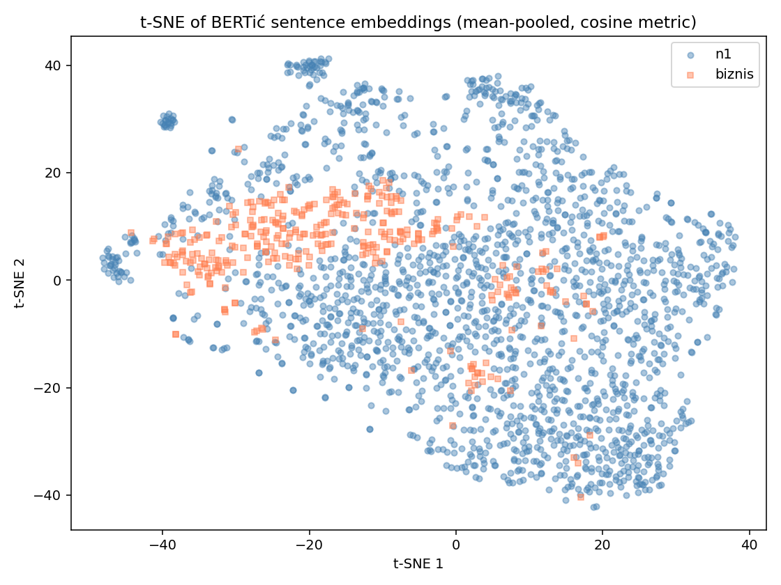A two-dimensional t-SNE projection of frozen BERTić embeddings. It is an illustration of local geometry, not an independent performance result.

One headline, two outlet prefixes

The final experiment fine-tuned google/mt5-small on (outlet + title) -> article body pairs. At inference, the same headline was sent through the model twice. Only one token changed:

This was not an attempt to automate journalism. I wanted to turn the classifier around. Classification asks whether outlet information is present in an article; conditional generation asks whether the same information is usable as a control. If one prefix changes the vocabulary while the headline stays fixed, the model has learned at least some directional association with the outlet label.

def make_input(source: str, title: str) -> str:
    prefix = "n1" if source == "n1" else "biznis"
    return f"{prefix}: {title}"

In mathematical shorthand:

$$x=\texttt{<outlet>: title}, \qquad \texttt{<outlet>}\in\{\texttt{n1},\texttt{biznis}\}.$$

Across 150 generated samples, switching from the n1: prefix to biznis: nearly doubled the presence of Biznis-specific markers, from 29.3% to 57.3%.

One control token changed the generated vocabularyShare of 150 samples containing Biznis-specific markers

n1: prefixBiznis markers in generated text

29.3 %

biznis: prefixBiznis markers in generated text

57.3 %

That is evidence that the control prefix changed the generated vocabulary. It is not evidence that the model could write publishable news. The 300M-parameter model frequently produced poor Serbian grammar and invented names, dates, and numbers. Real/generated top-word overlap was only 4/50 for N1 and 0/50 for Biznis. The result is a controlled representation experiment, not a newsroom product.

What I take from the project

The project made me more skeptical of impressive first results. When a simple model reaches the high nineties, the productive response is not immediately to replace it with a transformer. It is to look for shortcuts, rebuild the evaluation boundary, and ask which parts of the data made the task easy.

It also reinforced a preference for small models as investigative tools. Logistic-regression coefficients, low-rank components, ablations, and deliberately constrained generators each answered a different question. Together they produced a better account of the corpus than any single leaderboard number.

Most importantly, the scraper and the analysis are one system. Collection choices determine the claims the model can support. A missing paragraph, repeated wire copy, retained byline, or one-month sampling window is not merely a data-cleaning detail; it becomes part of the model's behavior. The system is trustworthy only when those choices remain visible from collection through evaluation.

What I would change next

The next version should make the evaluation stricter before making the model larger:

1. Fit TF-IDF, LSA, and every learned transform inside each training fold.
2. Deduplicate syndicated or near-identical articles and group related stories into the same fold.
3. Hold out a later month to measure temporal generalization.
4. Add more outlets and match articles by topic so editorial style can be separated from beat selection.
5. Treat generation as a retrieval-grounded, human-evaluated task or leave it out entirely.

The strongest conclusion is modest: simple lexical models captured nearly all measurable source signal, compression preserved most of it, and careful ablation was more informative than adding model complexity.

View the source on GitHub